The VLOOKUP function is used to return a value from one place in your spreadsheet into the cell where the VLOOKUP function sits. If you live your life in spreadsheets, it’s just a matter of time before you hear about how INDEX MATCH is preferred by some over the use of VLOOKUP.
Given the two alternative approaches can produce the same result, the basis on which they are being compared here is one of performance, namely speed of calculation. This comes into play in a noticeable manner if your model is large (a dozen+ sheets, hundreds of columns, hundreds of rows of calculations on many of them) and it includes circular references.
Using INDEX MATCH in the place of VLOOKUP
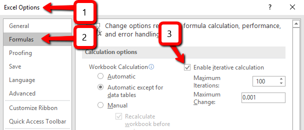
If your model includes circular references, to get it to calculate, you will have to enable iterative calculations in the file (File > Options)
Let’s say that your file currently includes a slew of VLOOKUP-based formulas and you want to replace them with INDEX/MATCH-based formulas.
Here’s how to do it in a generic manner:
Existing VLOOKUP-based formula:
=VLOOKUP(lookup_value,table_array,col_index_num)
Equivalent INDEX/MATCH-based formula:
=INDEX(right-most column range of table_array,MATCH(lookup_value,left-most column range of table_array))
A practical example of replacing VLOOKUP with INDEX MATCH
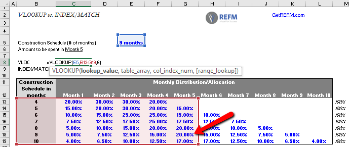
Let’s say we have a lookup table for construction hard cost spend allocation over the months of a variable-length construction schedule (a construction “bell-shaped curve”). And let’s say we want to know what % of the total budget is spent in Month 5 of the construction schedule.
VLOOKUP implementation
To set this up using VLOOKUP, we reference the lookup value of 9 months in cell E5, define the table array starting at column B and extending through column G (that of Month 5), and then provide the number of column movements into the table. The value it pulls back in this case is 20.00% (the one in cell G18).
INDEX/MATCH implementation
If we wanted to return this same result using INDEX/MATCH instead of VLOOKUP, we can construct the compound function as shown in cell C9 below:
=INDEX(Just column G of the prior-defined array, MATCH(lookup value in E5,Just column B of the prior-defined array))
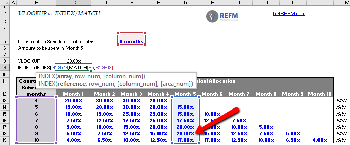
In this implementation, the same 20.00% value in cell G18 will be returned.
Comparison of the two approaches
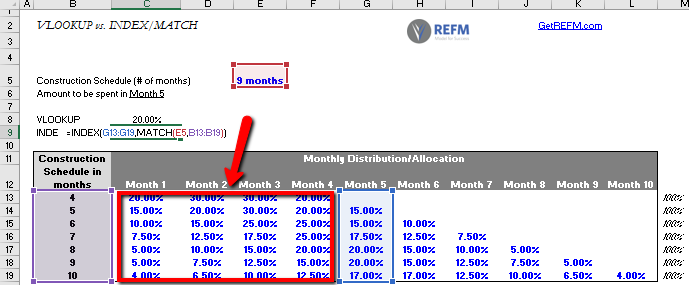
The fundamental difference between these two formulas is pretty evident — in VLOOKUP, the entire set of columns from the lookup value column through the sought-value column is scanned through by Excel, whereas in INDEX/MATCH, Excel is only scanning the two columns with which it is provided (the red boxed area shown below is purposefully ignored by INDEX/MATCH).
When it makes the most sense to use INDEX MATCH over VLOOKUP
In a small, relatively simple file, there won’t be any noticeable difference in speed of calculation for the worksheet or workbook, but in a complex, circular reference-laden file, INDEX/MATCH can save you time every time calculations run.
Additionally, it makes sense to use INDEX/MATCH when you know the column you’re seeking, and you know that that column will remain the one in which you’re seeking the value. In the example above, we know we want to pull the Month 5 percentage value, so our formula focuses on that column.
VLOOKUP is the solution to apply if the sought-value column is subject to change. An example of this is if you wanted to pull all the individual scheduled percentages into a row (each month’s percentage into its own cell), not just pull the percentage for Month 5 into a single cell.
All of REFM’s Excel model templates are optimized for speed by avoiding circular references in the first place. They’re lightning fast, literally zero waiting for calculations.
The file is embedded below. You can download it by clicking on the download icon in the bottom border of the embed window.