Unfortunately for us, Excel requires that literally every new tab we create be formatted from scratch. It’s pretty awful and painstaking work with which we are all too familiar. In some cases we might find ourselves spending up to 15% of our time just making our spreadsheets look presentable for their audience. The sad reality is that humans subconsciously superficially judge the value of something presented to us based on its appearance.
One of the ways that we can put the odds in our favor for a positively biased reception of our work is to keep it meticulously clean. Less is more in presentation, but the challenge is that less is always harder to do than more. One of the tricks that I have found can help is to use Excel’s conditional formatting to make extraneous elements disappear from view.
For example, if you have an apartment acquisition Excel template that contains an exhaustive unit mix table capable of summarizing the composition of pretty much any building’s rent roll, you can use conditional formatting to prevent the irrelevant unit type line items from displaying altogether, keeping the presentation free of distracting noise.
Without using conditional formatting, here’s how a unit mix table might look:
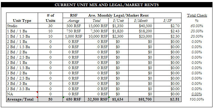
See all the rows that have zero units each? Now look at the table when there is conditional formatting that hides all entries in rows for which the number of units = zero.
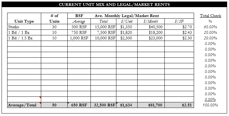
Much better, right?
Here’s how you accomplish this higher level of presentation easily:
- Highlight one of the rows where you want values to potentially not be displayed if they are not relevant (e.g., the top row in the table above)
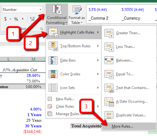
- Go to the Home tab, and select Conditional Formatting in the Styles section, and then Highlight Cells Rules, and then More Rules
- Type in the custom rule (in this case, when the # of Units column value = 0) and then select Format (be sure to not have any cell anchoring in the cell coordinates)
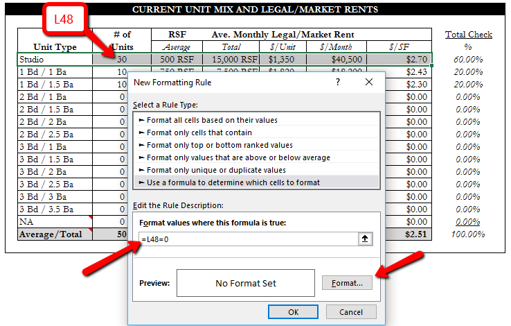
- Select the format that will result in the values disappearing (in this case, since the sheet background is already painted white, simply change the Font Color to white)
- Click OK and then click OK again
- Then select the row area again and click on the Format Painter icon in the Home tab under Clipboard
- Paint the format onto all other rows for which you want the formatting to apply.
That’s it! Please put any questions below.
If you are looking for a great back of the envelope calculator for apartment property acquisition, see our free tool here.
You can find robust projection templates here.