|
Listen to this post if you prefer
|
One of the headaches we face in underwriting multi-family assets is distilling the (sometimes massive) rent roll into a more manageable unit mix summary table. Luckily, we have the UNIQUE function to make relatively quick work out of this task, and then we can perform analysis on the table by leveraging SUMPRODUCT and SUMIF.
The UNIQUE function applies to a data range/array and returns a list of unique values, ignoring duplicates. Due to its ease of application on large data sets and its ability to simplify these data sets, UNIQUE is a powerful summary tool for dynamic lists.
The full syntax of the UNIQUE function is:
=UNIQUE(array,[by_col],[exactly_once])
where array is the only required argument in the formula, and by_col and exactly_once are optional arguments.
By nature, UNIQUE is a dynamic array function. This means that any additional unique values will populate or spill into adjacent cells when there is more than one unique value in a data set, so keep adjacent cells clear when using the formula.
Let’s start with a description of two different basic applications of the UNIQUE. You can follow along in the Excel file here.
Unique Values vs. Only Values Occurring Once
Assume that you have a large array of inputs from a rent roll and want to create a dynamic summary table that pulls distinct values from it.
The most basic syntax for the UNIQUE function is as follows:
=UNIQUE(array)
This syntax will produce an exhaustive list of the unique values in the overall array being evaluated, whether each value occurs once or more than once.
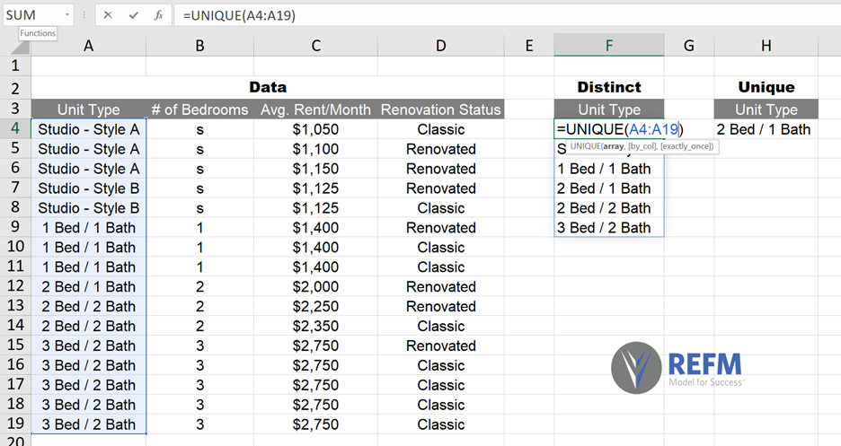
In the example above, the UNIQUE formula takes the data set in column A and lists every unique value once in the order that it appears from top to bottom of the array. To be clear, when using the UNIQUE function, it is only necessary to type the formula into one cell (in our example above, cell F4) and then Excel will automatically propagate that same formula vertically downward for however many cells are needed to show all unique results in the data set. We note that the formula in the cells below the original cell will be grayed out in the formula bar when they are selected.
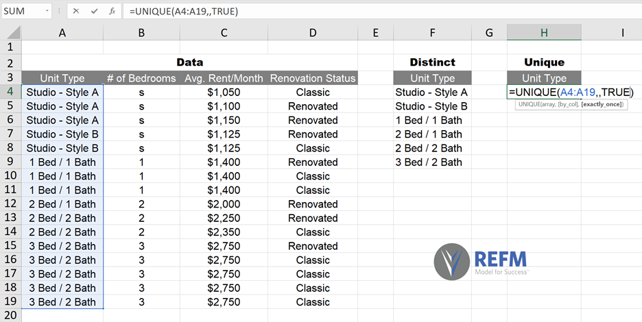
If you want to only see the unique values that occur only one time in the data set, then you can use the following syntax, inserting TRUE in the [exactly_once] argument place: =UNIQUE(array,,TRUE)
This is shown in cell H4 of the image below, which shows “2 Bed / 1 Bath” as the only result (see H4 in the graphic above), as that unit type is the only one that shows up just once in the overall rent roll array being evaluated.
Applying UNIQUE by rows vs. columns
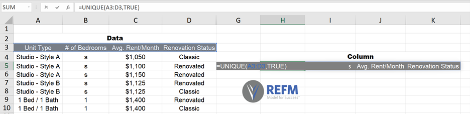
By default, the UNIQUE function will evaluate a vertical array (i.e., an array of disparate rows in the same column) and “spill” its results into multiple cells in the rows below the cell in which the originally-typed formula exists.
If you desire instead to pull data that spans multiple columns of the same row, then type TRUE or 1 in the second argument of the UNIQUE function [by_col] as follows: =UNIQUE(array,TRUE)
In the graphic below, the formula is entered in cell H5, and propagates the unique column headers from A3:D3 into cells H5:K5.
Using UNIQUE with multiple criteria
In the case where you would like UNIQUE to filter and extract data based on two criteria, an “&” may be used in between two sets of data. For example, if you wanted to produce a list of units that separated out not just the unit type, but also the renovation status of that unit type, you could do so as we show below in cell G13.
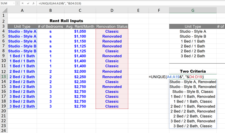
Excel automatically produces the exhaustive list and separates the criteria with a comma.
Rent Roll-to-Unit Mix Summary Table Examples
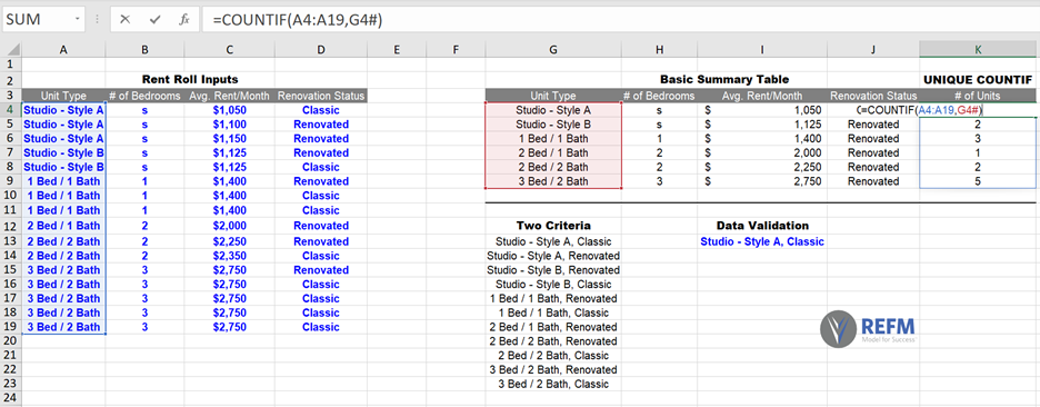
The UNIQUE function is especially valuable when it is paired with a reference-based function such as =INDEX(MATCH)), SUMIF, or COUNTIF to create a rent roll summary table with data being grouped by each specified unique value.
The example graphic below shows a column of data in column H for the # of Bedrooms, based on the Unit Type list generated by UNIQUE in column G.
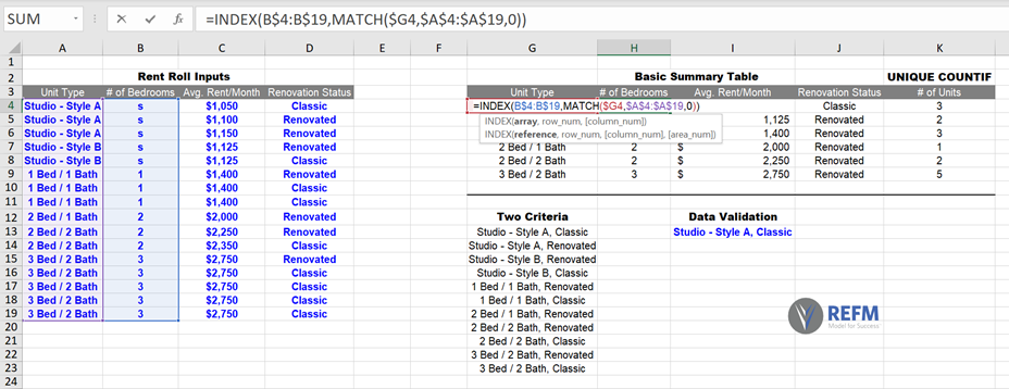
The example graphic below shows a column of data in column K for the # of Units of each Unit Type using COUNTIF. The # symbol immediately following G4 means that COUNTIF() will be applied to all unique values in the list, even if more are added in the future. This is very effective when combined with the UNIQUE function, as added unit types will be processed in the same manner as the existing ones.